The campaign against ‘nonsense’ output gaps

The debate on the output gap is hardly new. What motivates this review is rather the social media campaign Robin Brooks (Institute of International Finance) recently launched against “nonsense” consensus output gaps (#CANOO) in the euro-area periphery. We review the economic argument, the direct responses, and some less recent pieces related to the output gap and its measurement.

First, some background remarks: the output gap refers to the difference between actual GDP and an unobservable measure of its ‘potential’. So the debate is really about defining and accurately estimating potential output (and its growth).

By referring to consensus, Brooks points to the three organisations that routinely produce output-gap estimates for advanced economies: the European Commission, the International Monetary Fund (IMF) and the Organisation for Co-operation and Economic Development (OECD). According to the consensus, potential is defined as a supply-side constraint on output – the point where the economy operates at full capacity. Seen from a production-function perspective, potential output is a measure of economic slack or underutilisation of its production factors (e.g. labour). Similarly, it can be interpreted as the level of output in which additional demand only results in inflationary pressures, hence its use in steering monetary policy. The identification of the cycle is also why potential output is used to calculate the structural fiscal balance.

Brooks and Greg Basile (here, here and here) argue that, seen from a cross-country perspective, output gaps in the euro-area periphery are implausible. Their premise is that countries with strong real economic growth per capita in the last decade cannot have the same output gaps as countries with negative per-capita economic growth. For instance, Germany and Spain are estimated to have roughly equal output gaps despite real per-capita GDP growing more than 10% since 2007 in the former while remaining nearly constant in the latter (Figure 1, left); a similar discrepancy is reported for Australia and Italy.

Figure 1

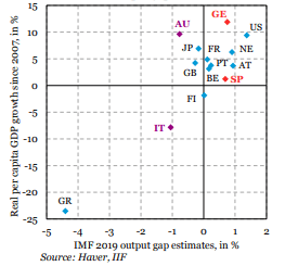
Source: Brooks and Basile.

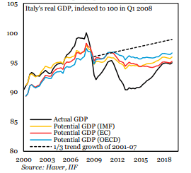
To support their argument, Brooks and Basile point to the Phillips curve. Despite decreasing or zero slack, core inflation remains low (Italy for example, see Figure 2, left). They suggest that the measure of underutilisation is wide of the mark; they point out, for instance, that the unemployment gap for Spain and Portugal is roughly the same as in Belgium (Figure 2, right).

Figure 2

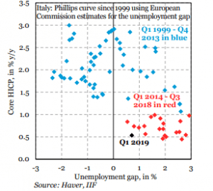
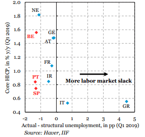
Source: Brooks and Basile.

At the heart of Brooks‘ and Basile’s criticism is the “pro-cyclicality” of potential output estimates. As they put it, “the underlying problem is that these numbers don’t capture “potential”, but “seem to be more about capturing realized outcomes over the last decade”. The concern about the pro-cyclicality of output-gap estimates is shared by other commentators. For example, Philipp Heimberger shows that “for the euro area group of countries there is almost a perfect positive correlation between changes in potential output and changes in real GDP (calculated in relation to the pre-crisis growth trend)” (Figure 3).

Figure 3

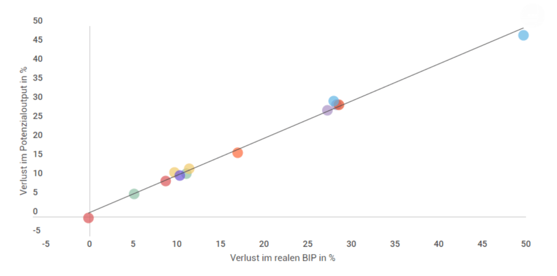
“y = 0,9735x + 1,0571; R² = 0,9939. Data: AMECO (May 2019 update); own calculations. The group of countries includes 13 euro area countries, although some countries could not be included in the pre-crisis estiamtes of potential output due to data problems. For details on the method of calculating losses in potential output and real GDP: see Heimberger, P.; Kapeller, J. (2017): The performativity of potential output: Pro-cyclicality and path dependency in coordinating European fiscal policies, Review of International Political Economy, 24(5), S. 917

Source: Philipp Heimberger.

Further, Adam Tooze points to the statistical techniques used to separate the structural from the cyclical component in the labour markets as the main culprit. He explains, for instance, that the Commission’s estimation of the long-term sustainable growth of employment and productivity entails a statistical technique known as a Kalman Filter, which “in layperson’s terms this is roughly equivalent to a rolling average of past performance”. This is the direct channel of pro-cyclicality: potential GDP is essentially a moving average of past economic outcomes and mechanically “bends-down” when theses outcomes are bad (and vice versa).

The problem of separating the cyclical from the structural is especially challenging during a crisis due to so-called “hysteresis” effects, as critics of the current methodologies also acknowledge. In Heimberger’s words, “the concept of hysteresis assumes that insufficient demand in times of crisis can have long-term effects on the supply-side potential of an economy, e.g. when long-term unemployment leads to skill losses of people who have become unemployed as a result of the crisis”.

Nevertheless, in some cases consensus output gaps mean negative trend growth for potential output, an assumption which Brooks and Basile describe as “extreme”. To illustrate that, they construct their own potential output alternatives using simple, ad-hoc assumptions. Based on the hysteresis premise, Brooks and Basile assume a 5% permanent drop in 2008 followed by positive, yet lower, potential GDP growth thereafter (1/2 for Portugal, 1/3 for Italy and Spain and 1/10 for Greece) compared to the pre-crisis trend. Their derived output gap differs substantially to the other organisations’ estimates (shown in Figure 4). Heimberger, makes a nearly identical assumption about Italy (without the 5% permanent drop) and also finds a large discrepancy (Figure 5).

Figure 4

Source: Brooks and Basile.

Figure 5. Potential output (YPOT) and real GDP in Italy

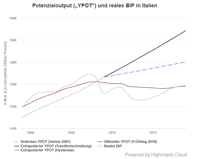
“Data: AMECO (autumn 2007 and spring 2019 update); own calculations. YPOT (note: dotted line): potential output; trend update: extrapolation of the pre-crisis YPOT with the average potential growth rate of the years 2000-2009 (based on the Commission estimate in autumn 2007) for the years 2010-2019 (note: solid black line); hysteresis: extrapolation of the pre-crisis YPOT taking into account significant hysteresis effects in the sense of a constant potential growth rate of 0.5% in the period 2010-2019 (note: solid blue line)”.

Source: Philipp Heimberger.

Notes: Official potential output (spring 2019) - solid red line; real GDP - solid grey line

Italy’s output gap has been the central theme in the response to the “nonsense” output gap campaign, given the implications it has on fiscal policy under EU rules. The table below (Table 1) by Heimberger shows what different output-gap estimates imply for the fiscal policy stance of Italy in 2019 relative to its structural target in the medium term (−0.5% of GDP).

Table 1. Figures for Italy (2019)

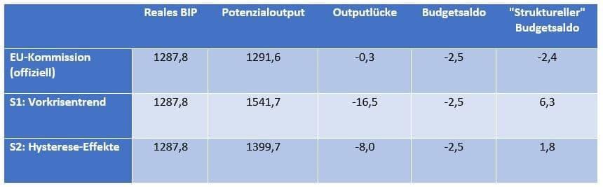
“Comments: Real GDP and potenetial output in billions of € at constant 2000 prices. Budget balance and “structural budget balance” in % of GDP. Data: AMECO (May 2019 update); own calculations.”

Source: Philipp Heimberger.

Scott Sumner, for example, asserts that if potential is interpreted as a counterfactual under appropriate economic policy (including more efficient taxes, spending, regulations, etc.) then Italy’s output gap is indeed large, and has widened in the past decade. But he notes that, ultimately, what this reflects is the “structural”, not demand-related, problems Italy faces, implying the need to implement the appropriate economic policies.

But in their columns, Heimberger and Tooze suggest another, indirect channel for the pro-cyclicality of potential output: flawed output gaps combined with EU fiscal rules can constrain demand, thus leading to inferior actual economic outcomes ex post. This is not to say, however, that either one of them suggests fiscal expansion would resolve Italy’s structural challenges – which they acknowledge; rather, the argument is that fiscal consolidation as suggested by the output gap was and will remain counter-productive.

Fabio Ghironi weighs in, agreeing that there is a problem about how output gaps are constructed. He also accepts the possibility that potential “bends down” because it incorporates the results of past policy mistakes. Hence, “it is legitimate to ask whether, in estimating potential (or a range of possible paths for potential), we should also account for the possible effects of corrective policy actions that would (at least to some extent) undo the effects of past mistakes on potential”. He cites research suggesting aggregate demand can have an impact on potential supply through investment, R&D and technology adoption – in his view Italy’s most pressing economic problems. Ghironi writes, however, that the current deficit spending plans of the Italian government are not significantly growth-enhancing, by its own admission. So, rather than alleviate Italy’s structural economic issues, these plans will worsen its credibility problem.

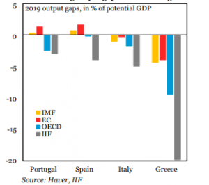
The use of output gaps in crucial policy decisions in the EU points to the need for accurate estimates in real time. However, Zsolt Darvas demonstrates the large degree of uncertainty that surrounds these estimates. For one thing, even the range of estimates between the three international organisations is very large (Figure 6), not to mention the range of the confidence intervals around them. For another, the estimates of both the output gap and consequently the structural balance are subject to large revisions. Crucially, Darvas’ calculations show that the uncertainty around the estimates today is not lower than it was during the crisis.

Source: Zsolt Darvas.

Given that the output gap guides fiscal and monetary policy around the world, naturally the question follows as to whether it is a reliable measure at all?

In addition to its empirical problems, Chris Dillow raises some theoretical criticisms of the output gap. Citing microeconomic studies, he argues that capacity constraints may lead to productivity gains, rather than price hikes. He adds that high demand may lead to price cuts to capture customers and maintain them in the future (especially when interest rates, and thus discount factors, are low). Finally, capacity limits do not readily apply to the intangible economy due to scalability, so the output gap might be even less of a relevant concept going forward.

In the context of deciding monetary policy, Stephen Millard favours a measure of real marginal cost relative to equilibrium or desired levels over the output gap as a proxy of inflationary pressures. He lists two reasons why the supply constraint of an economy may not coincide with an inflation-neutral level of output. First, because of real frictions, such as lack of competition leading rent-seeking behaviour. Second, because in an open economy resources are not fixed, i.e. they can be imported (e.g. migration of workers). Millard maintains that with minimum assumptions, the observable labour share of gross output (relative to its average) is equivalent to real marginal cost. Given, however, that the empirical evidence for this variable is mixed he suggests that directly surveying firms about their margins (and their desired levels) is a viable alternative.

Yvan Guillemette and Thomas Chalaux of the OECD, on the other hand, make a case about how the current empirical methodology can be improved. They ran a regression of actual growth on revised (not real time) vintages of output gaps and found that European Commission series were the most cyclical, followed closely by IMF estimates, whereas the OECD coefficient is less than half of the two others (Figure 6 – higher coefficients corresponding to more pro-cyclical estimates). They go on to suggest that “one reason the OECD potential output measure may be less cyclical is that before smoothing them with a filter, the component series used to construct potential output are first cyclically adjusted by making use of other variables – such as survey measures of capacity utilisation or the investment rate – which are known to be correlated with the cycle (see Turner et al., 2016)”.

Figure 7

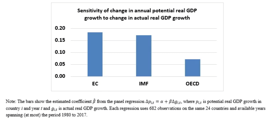
Source: Yvan Guillemette and Thomas Chalaux.

Finally, considering financial variables in the estimation of output gaps is another promising approach. Caludio Borio, Piti Disyatat and Mikael Juselius, for instance, showed that “finance-neutral” output gaps, which incorporate information from variables that proxy the financial cycle, are much more precise and, above all, are much more robust in real time (for Spain, the UK and the US).

At least two similar studies summarised in blogs reach the same conclusions: David Arseneau’s and Michael Kiley’s, introducing measures of credit or house-price developments into a traditional empirical model of output gap with labour-market slack for the US; and Marko Melolinna’s, running a semi-structural unobserved components model and including the so-called Financial Conditions Index (FCI) for the UK.